

Sometimes to choose the appropriate model, the suitable training algorithms, and the hyperparameter to best fit the task as well as to debug issues and perform error analysis more efficiently, it is necessary to understand what is under the hood when applying Linear Regression.
Hence, in this post, we will dissect the implementation of linear regression using Matlab. Linear regression is a statistical algorithm used in machine learning, as a supervised learning technique to predict a real-valued output based on an input value.
For this analysis, we selected a free and publicly available dataset from a well-known data source. It contains a house, lot area, year of build, bedroom avg, and many more features. Also, we use vectorization which is more efficient than for loops because of its parallel computation capability.
Linear Regression with One Variable
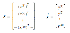
It is important to establish the notation for this analysis, where we’ll use \(x^{(i)}\) to denote the input features, and \(y^{(i)}\) to denote the target variable that we are trying to predict from a data set. A pair (\(x^{(i)} , y^{(i)}\)) is the training example. The dataset used to learn as a list of m training examples \({(x^{(i)}, y^{(i)} ); i = 1, . . . , m}\) is a training set.
Bear in mind that the superscript \({(i)}\) in the notation is an index of the training set instead of the exponentiation. We will also use X to denote the input values and Y as the output values, both as real numbers ℝ.

Hypothesis and Cost Function (MSE) for One Feature
In supervised learning problems, the goal is, given a training set, to learn the hypothesis \({h: X → Y}\) so that \({h(x)}\) is a valid predictor for the corresponding value of continuous y, known as a regression problem.

We can measure the accuracy of our hypothesis by using the “Squared error “/ “Mean squared error” cost function. The idea of this function is to choose $latex \theta_0$ and $latex \theta_1$ so that $latex {h_\theta(x)}$ it is close to \({y}\) for the training example, where the value of $latex J(\theta_0, \theta_1)$ will be 0. The MSE is a convex function where we will have only a global optimum in contrast with other functions where we could end in local optima.

Thus as a goal, we should try to minimize the cost function. To implement this cost function in Matlab, first, we need to get the size of the X matrix stored in variable m. In addition, it is necessary to pass additional hyperparameters. In this case, the X corresponds to the matrix containing all features input.
The theta vector is the same size as the number of X input features, and finally the vector y correspondent to the labeled output values.

Matlab is a computer numerical program, that interprets the operator “*” as the multiplicator for two matrices. So, if we want to multiply a scalar value to a matrix, vector, or another scalar, we need to add a “.*” before each operator as we did in the computation of the exponential of \({(h(x) – y)^2}\), while element-wise multiplication. Also, we can use a series of pre-built functions as we did use the sum() function.
Batch Gradient Descent for One Variable
Now with the hypothesis function, we have a way of measuring how well it fits into the data. Therefore, we need to estimate the parameters in the hypothesis function. That’s where gradient descent comes in.
When specifically applied to the case of linear regression, a new form of the gradient descent equation can be derived. We can substitute our cost function and our hypothesis function and modify the default gradient descent equation to :

where m is the size of the training set, $latex \theta_0$ a constant that will be changing simultaneously with $latex \theta_1$ and \(x_{(i)}, y_{(i)}\) are values of the given training set.
If we start with a guessing point for our hypothesis and then repeatedly apply these gradient descent equations, our hypothesis will become more and more accurate. So, this is simply gradient descent on the original cost function $latex J$. This method looks at every example in the entire training set on every step and is called batch gradient descent.

To compute the batch gradient descent, some additional useful hyperparameters are needed. Essentially the number of iterations and the learning rate alpha.
You may want to adjust the number of iterations. Also, with a small learning rate, you should find that gradient descent takes a very long time to converge to the optimal value (underfitting the training set), on the other hand with a large learning rate, gradient descent might not converge or might even diverge (overfitting the training set).
Also, bear in mind that theta should be updated simultaneously after the computation of temporary theta on each iteration.
Linear Regression with Multiple Variables
Linear regression with multiple variables is also known as multivariate linear regression. For multiple variables, our notation differentiates slightly from the initially presented one. Now we can have any number of input variables.

Linear Regression – Hypothesis and Cost Function (MSE) for Multiple Features
Using the definition of matrix multiplication, our multivariable hypothesis function can be concisely represented as:

We can think about $latex \theta_0$ as the basic price of a house, $latex \theta_1$ as the price per lot area, $latex \theta_2$ as the price per bedroom…. \({x_1}\) will be the number of lot area in the house, \({x_2}\) the number of bedrooms and so on.

The vectorized version is:

where
For convenience we assume $latex x_{0}^{(i)} =1 \text{ for } (i\in { 1,\dots, m } )$, allowing us to do matrix operations with $latex \theta$ and \(x\), making the two vectors match each other element-wise.

As well in the linear regression with one variable, the only difference is the number of the input value features and the number of theta that is proportional to the number o feature X matrix.
Notice too that in the vectorized version of the hypothesis, we need to transport the theta. We did this by inverting the order of the multiplication of X*theta. This is the same as theta’*X since suppose our matrix X is 10×4 and the vector theta must be 4×1. Thus we are multiplying matrices of compatible dimensions where collum X is equal to the row theta.
Linear Regression – Batch Gradient Descent for Multiple Variables
The gradient descent equation for multiple variables is generally the same. We just have to repeat it for our n features.

Vectorized matrix notation of the Gradient Descent:

It has been proven that if the learning rate α is sufficiently small, then $latex J(\theta_0)$ will decrease on every iteration. For sufficiently small $latex \alpha$, $latex J(\theta)$ should decrease on every interaction otherwise If $latex \alpha$ is too small: gradient descent can slowly converge.

Feature Scaling and Mean Normalization
Gradient descent works faster when each of our input values is in roughly the same range. This is because $latex \theta$ will descend quickly on small ranges and slowly on large ranges.
We can normalize our set using Feature Scaling. It involves dividing the input values by the range of the input variable, resulting in a new range of just 1.
−1 ≤ $latex x_{(i)}$ ≤ 1
Feature scaling can be used with Mean normalization. Mean normalization involves subtracting the average value for an input variable from the values for that input variable resulting in a new average value for the input variable of just zero.

To implement both of these techniques, we need to adjust our input values where $latex μ_i$ is the average of all the values for feature $latex {(i)}$ and $latex s_i$ is the range of values or the standard deviation.

To perform these technics, first in MATLAB, we can use the mean and std functions to compute the mean and the standard deviation for all the features. The standard deviation is a way of measuring how much variation there is in the range of values of a particular feature.
Normal Equation as an alternative to Gradient Descent
Gradient descent gives one way of minimizing $latex J$. Another way to do this explicitly and without resorting to an iterative algorithm is by using the “Normal Equation” method. We minimize $latex J$ by explicitly taking its derivatives concerning the $latex \theta_j’s$, and setting them to zero. This allows us to find the optimum theta without iteration:

When we are using the standard equation we do not need to do feature scaling. With the standard equation, computing the inversion requires much more big $latex {O}$ time. So if we have a very large number of features, the standard equation will be slow and we should choose the iterative process.
We can tackle the problem of a non-invertible matrix by using regularization.

Also just for reference, beyond using the normal equation we can use another more complex and advanced mechanism to minimize $latex J$. These are MATLAB built-in functions called fminunc and fmincg.
Conclusion
In this article, we dissected the implementation of linear regression using Matlab since the importance of establishing a notation, and the use o linear regression for one variable, or multiple variables. We also reveal how Bacht Gradient Descent is used to estimate the parameters in the hypothesis function as well as the use of Feature Scaling and Mean Normalization to normalize our input values in roughly the same range.
Finally, we examine the use of Normal Equation as an alternative to Gradient Descent as well as a more complex and advanced mechanism like MATLAB built-in function fminunc and fmincg to minimize J.
The sample is accessible from the GitHub repository; to download it, please follow this link.